Beginning to study Unit 3 in QCAA Physics but aren’t too sure about what kind of content you’ll be covering? We’ve got you!
We want to make studying for this unit much easier for you, so we’ve broken down what each of the topics you’ll study involve and the different concepts you’ll be learning.
Ready to find out what’s covered in QCAA Physics Unit 3? Check it out!
What is Unit 3 in QCAA Physics all about?
Topic 1: Motion
Topic 2: Electromagnetism
What is Unit 3 in QCAA Physics all about?
Before we start, it is important to understand where Unit 3 sits in your overall knowledge of Physics. Grade 12 Physics is designed in such a way as to teach what is known as ‘classical physics’ during Unit 3.
Classical physics is what makes up our baseline understanding of the physical world and is more than enough to explain the large majority of what we observe on a daily basis.
It should be noted that while this guide gives an overview of all the Unit 3 topics, you should take your own time to investigate each of these topics in-depth as there are many scenarios that you will encounter in Grade 12 physics that we won’t be able to cover here.
Topic 1: Motion
Before we get into the meat of the topic, we first need to explain what a vector is and how it works. If you have done Specialist Maths in Grade 11 you will already know this but it’s nice to recap it anyway. Below is an image of a vector:
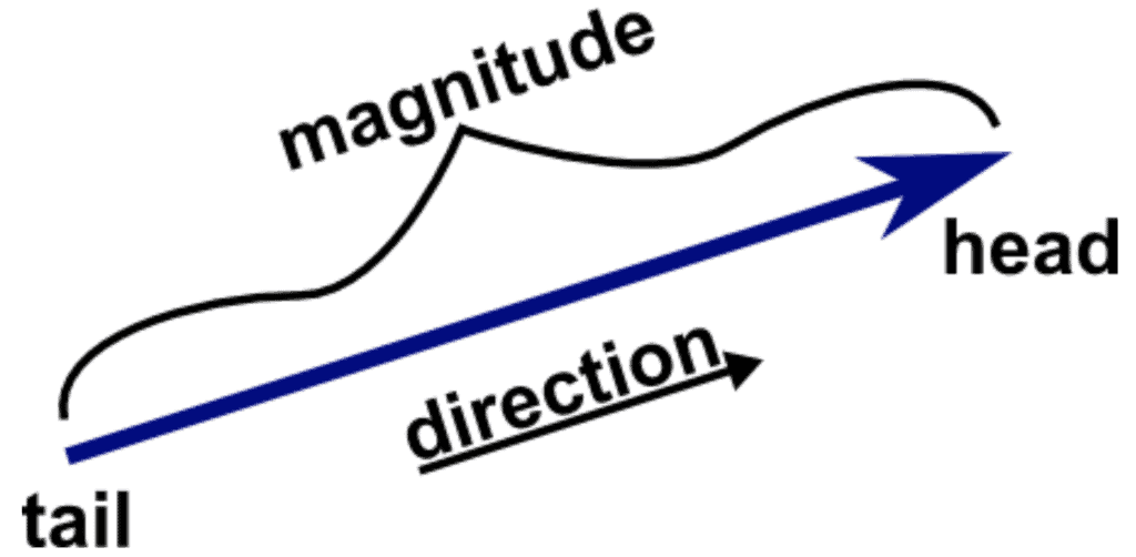
Image sourced from Math Insight
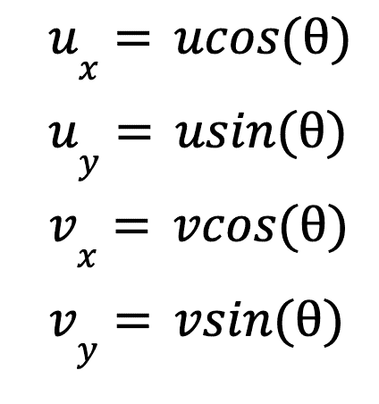
You can see from this that the vector is travelling both horizontally and vertically. Without getting too much into derivations, you will learn that the horizontal and vertical components respectively can be calculated as follows.
vx = Acos(θ)
vy = Asin(θ)
Where A is the magnitude of the vector and theta is the angle between the x axis and the vector. We can apply these equations to analyse the motion of objects which move according to these vectors!
Projectile Motion
At its most basic, projectile motion is a catch-all term describing a variety of situations. Let’s break down these situations from the most basic to the most complex.
The formulas we will need for projectile motion are as follows:
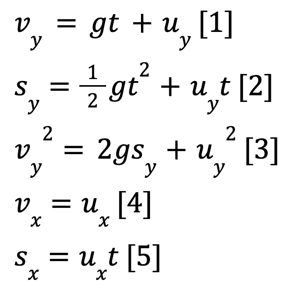
Where v is the final velocity, u is the initial velocity, s is the displacement and t is the time since the beginning of the projectile motion.
Projectile Motion Case 1: Horizontal Projection from a Height
Let’s consider a situation where you have a ball on the top of a cliff that is some height H.
If you were to give the ball a push horizontally what shape would the path of the ball make as it falls? First, let’s assume that there is no air resistance or drag forces to make this easier for us.
The first step to solving this is to consider the forces. With our assumption we can rule out any forces in the x direction, meaning that the initial horizontal velocity remains constant throughout the object’s motion.
In the vertical direction, the only force is due to gravity, giving the ball a constant acceleration downwards. With these forces in mind we can now determine that the ball will travel in a parabolic path as seen below.
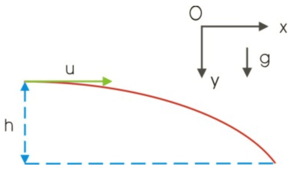
Image sourced from Tutor4Physics
From the 5 formulas we defined earlier, any parameter of this situation can be calculated. It is also important to note that due to the specifics of the situation uy = 0 as the ball is only given an initial horizontal push.
Projectile Motion Case 2: Projection at an Angle
This case is much the same as the first — however instead of being launched horizontally only, the ball is launched at an angle to the horizontal.
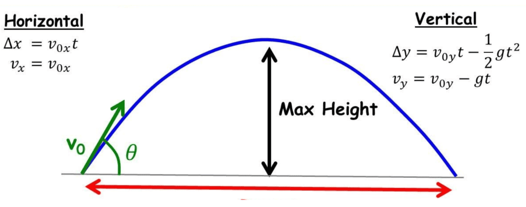
Image sourced from Physics Ninja
All the same equations apply here, the only difference is calculating ux, vx, uy and vy. Using the vector component equations that we mentioned earlier, we can determine:
A useful fact that you may need is that an angle of 45° will give the largest horizontal displacement. Similarly complementary angles will give the same horizontal displacements i.e sx(30°) = sx(60°)
Pause! We get this is a lot of content… that’s why it’s so critical to know how to take effective study notes in science – learn how!
Uniform Circular Motion
Have you ever spun a yo-yo above your head using its string? If so, then you have witnessed circular motion in action.
Now imagine spinning the same yo-yo at the exact same speed in the same way. This is Uniform Circular Motion.
The velocity of this spinning object can be described as v = distance/time where we know that the distance is the circumference of the circle it spins in, AKA distance = 2πr.
The time taken to complete a full revolution is the period and is represented by T. With these in mind the velocity can be expressed as v=(2πr)/T.
We should note at this point that the velocity vector is at all points tangent to the circular path that the object follows. The obvious question that follows from this then is what keeps the object moving in a circle rather than flying away?
This is answered through a concept known as centripetal acceleration represented by ac. This acceleration can be calculated as follows ac = v2/r.
This acceleration vector points towards the centre of the circle at all points. This combined with Newton’s second law allow for the calculation of the centripetal force, which is F = ma = (mv2)/r.
Gravity and Kepler’s Laws
One of the most important discoveries in physics is Newton’s description of gravitational attraction. It is as follows:
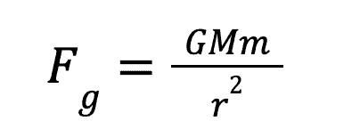
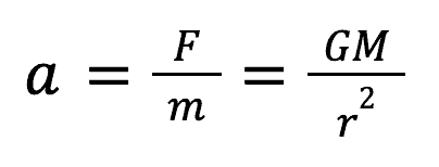
Where r is the distance between the two bodies, M and m represent the masses of the two bodies and G is the gravitational constant (given on formula sheet). Using Newton’s second law in combination with this expression, we can determine the gravitational acceleration at any distance from an object. It is as follows:
Another physicist known as Johannes Kepler expanded on Newton’s theories by using them to describe the orbits of planetary bodies. He came up with three main laws to describe these orbits.
The first law follows that planetary orbits are elliptical around the sun as the focal point. This went against the scientific consensus at the time that orbits were circular.
The second law follows that an orbiting planet will sweep out equal areas in equal periods of time — this one can be quite hard to understand before seeing a picture. See the below image which shows areas A1 and A2 being swept out over the same length of time. According to the second law, these areas are equal.
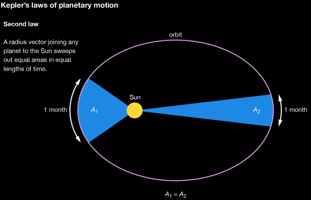
Image sourced from Brittanica
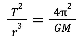
The third and final law states that the ratio between the square of the period and the cube of the semi-major axis is equal for all orbits. This can also be hard to understand when note seen in equation form. The mathematical description of this law is as follows:
Topic 2: Electromagnetism
Electromagnetic Forces and Electric Field
So far, we have mainly focussed on macroscopic situations, however, there is a whole other realm of microscopic situations which our current equations cannot describe. For this, we need to take a look into the equations of electromagnetism, starting with the electric field.
The basis of electromagnetism comes from Coulomb’s law, which states that the force between two charged particles is proportional to the product of the two charges and the inverse square of the distance between them. In equation form, this is:
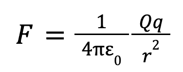
This equation explains why particles of the same charge repel each other and opposite charges attract each other.
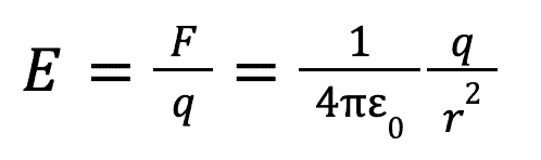
But why do particles experience this force? We know that for massive objects they experience gravitational forces due to a gravitational field that acts across a distance. From this we can speculate that something known as an electric field exists for charged particles which allows for this force to be exerted across a distance. This field can be calculated as follows:
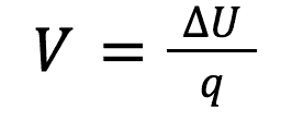
Potential Difference
The potential difference, commonly referred to as voltage is defined as the difference in potential energy between two points in a circuit, or in an electric field. Mathematically, it is defined as:
The Magnetic Field
Similar to electric forces having an electric field which allows for forces at a distance, magnetic forces act via the medium of the magnetic field. Unlike an electric field, the magnetic field is only produced by a moving charge.
There are a few different situations where the magnetic field applies in Grade 12 Physics. They are as follows:
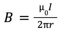
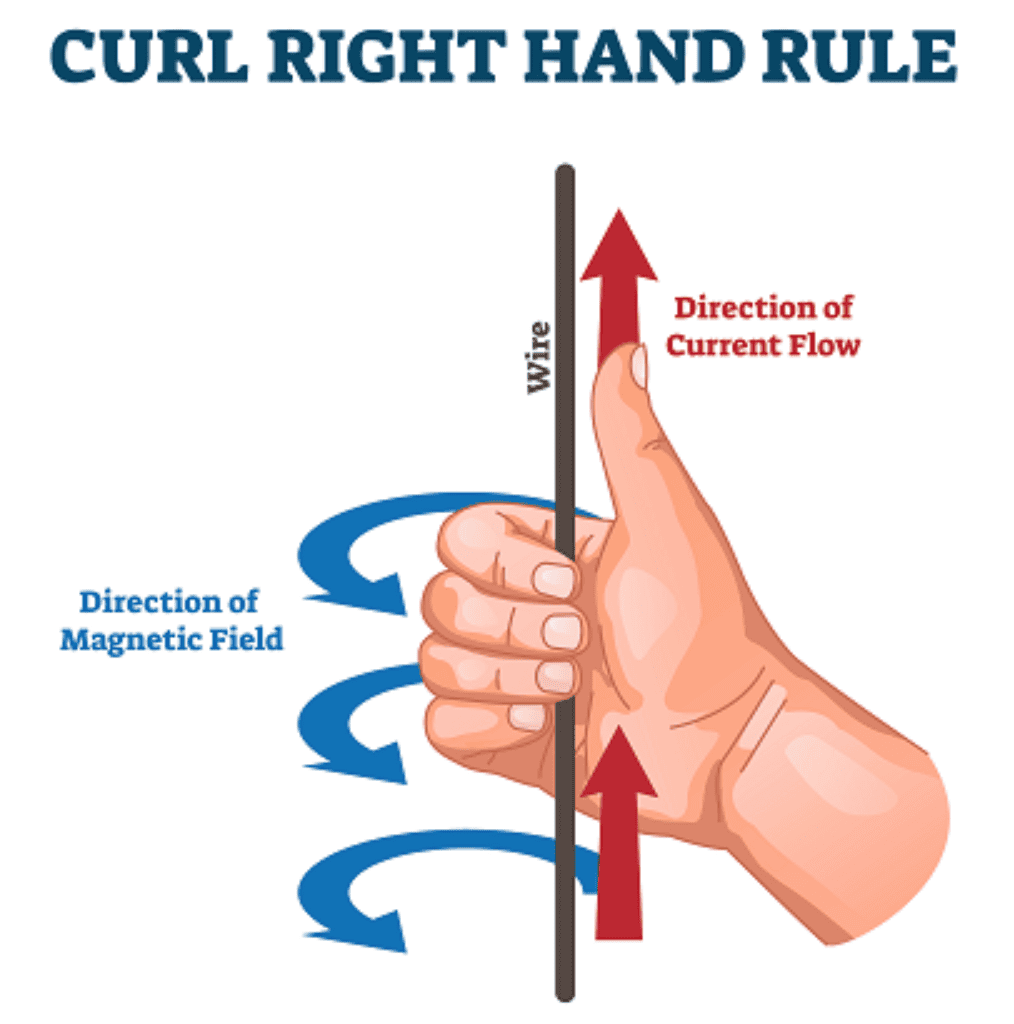
Around a current carrying wire
Where B is the magnetic field, I is the current flowing through the wire, r is the radius of the wire in meters and 0 is the magnetic constant given by the formula sheet. The direction of this magnetic field is given by the right hand rule which can be seen below.
Image sourced from Pasco
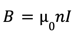
In a solenoid
Where n is the ratio of the number of turns in the solenoid to the length of the solenoid.
Magnetic Forces
Similar to the magnetic field, there are only a few situations in Grade 12 Physics where you need to be able to calculate a magnetic force, they are as follows:
For a current carrying wire in a magnetic field
F = BILsin(θ)
Where L is the length of the wire and theta is the angle between the magnetic field and the wire.
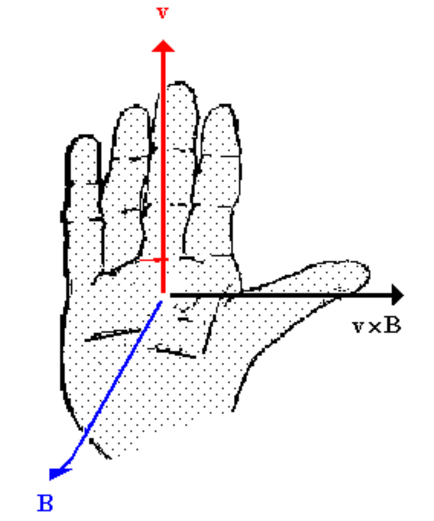
Magnetic force on a moving charge
F = qvBsinθ
Where q is the magnitude of the charge and v is the velocity of the charge. The direction of the magnetic force is dictated by the right hand rule which can be seen below:
Image sourced from Labman
Magnetic Flux
Magnetic flux can be described as the amount of magnetic field strength that is passing through a specific area. It is defined using the greek symbol phi and mathematically can be expressed as:
φ = BAcos(θ)
Electromagnetic Induction
Thinking back to our initial definition of a magnetic field, we said that it exists due to a moving charge, also known as a current.
Taking this idea we could theorise that a moving magnetic field would produce a current, this is correct and this theory has been measured empirically and we call this electromagnetic induction.
The Electromotive Force
Following on from the ideas of electromagnetic induction, if a current is created from a moving magnetic field, some work is done to move electrons — this work therefore creates an electric potential difference, or voltage.
We call this potential difference created by the magnetic field the electromotive force (emf for short). It is important to note that this isn’t really a physical force and the name is purely historical.
Mathematically, the emf can be described in terms of the changing magnetic flux through an area as follows:
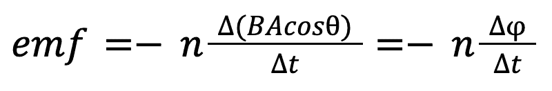
Where n is the number of turns, phi is the magnetic flux and delta (Δ) t is the amount of time passed in seconds.
Transformers
An example of electromagnetic induction that is important to understand is the idea of a transformer. At its most basic, a transformer is a device that transfers electrical energy from one circuit to another.
It does this by transforming its initial electrical energy into a magnetic flux which is then transformed back into electrical energy in a new circuit. The two circuits contain a different number of loops and therefore the voltage is also changed. The relationship between these are as follows:
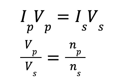
Where I represents current, V represents voltage and n represents the number of turns. The subscripts p and s represent primary and secondary, respectively, and are a way of representing either the primary or secondary coil of the transformer.
A transformer where the voltage decreases from the primary to secondary coil is known as a step-down transformer while a transformer where there is an increase in voltage is known as step-up.
Ready to kick on over to Unit 4? Check out QCE Physics Unit 4: Revolutions in Modern Physics, or bookmark it for later!
There you have it!
Know where you sit compared to your peers by using our new QCE Cohort Comparison Tool!
That’s everything you need to know for QCAA Physics Unit 3 summed up in an article. All the best with tackling your Unit 3 assessments!
We’ve got many practice questions for you to use to revise content throughout the year! Check them out:
- Unit 3 Physics Data Test IA1 Practice Questions
- Practice Questions for Unit 3 & 4 Physics External Assessment
- Multiple Choice Practice Questions for Unit 3 & 4 Physics External Assessment
- QCAA Physics Practice Exam
- What to Do if Your Real IA1 is at the End of Year 11
You’ll also want to have a look at our nifty guides for working on your QCAA Physics assessments below:
- The 9-Step Guide to Conducting a Student Experiment for QCAA Physics
- 7 Easy Steps You Can Follow to Complete a Research Investigation for QCAA Physics
- How to Ace Your External Assessment for QCAA Physics
Are you about to start Unit 4 of Maths Methods? Don’t miss this awesome content summary for you to use for your study!
Are you looking for some extra help with revising QCAA Physics Unit 3?
We have an incredible team of QLD Physics tutors and mentors!
Preparing to start Year 12? Don’t feel ready? Take this quiz to see how you’re tracking!
We can help you master the QCAA Physics syllabus and ace your upcoming Physics assessments with personalised lessons conducted one-on-one in your home or online!
We’ve supported over 8,000 students over the last 11 years, and on average our students score mark improvements of over 20%!
To find out more and get started with an inspirational QLD tutor and mentor, get in touch today or give us a ring on 1300 267 888!
William Bye is a Content Writer at Art of Smart and is currently studying a Bachelor of Advanced Science with Honours (majoring in Physics) at the University of Queensland. He was part of the very first cohort in Queensland to go through the ATAR system and wishes to help other students to make this journey as easy as possible. Will enjoys his time playing guitar in a band with his friends and hopes to continue balancing his science and music for many years to come.